Latest Posts by ocrim1967 - Page 4

The Shrinking Aral Sea

The Aral Sea was once the fourth-largest lake in the world. Fed primarily by snowmelt and precipitation flowing down from faraway mountains, it was a temperate oasis in an arid region. But in the 1960s, the Soviet Union diverted two major rivers to irrigate farmland, cutting off the inland sea from its source. As the Aral Sea dried up, fisheries collapsed, as did the communities that depended on them. The remaining water supply became increasingly salty and polluted with runoff from agricultural plots. Loss of the Aral Sea’s water influenced regional climate, making the winters even colder and the summers much hotter.

While seasonal rains still bring water to the Aral Sea, the lake is roughly one-tenth of its original size. These satellite images show how the Aral Sea and its surrounding landscape has changed over the past few decades.

For more details about these images, read the full stories here: https://go.nasa.gov/2PqJ1ot

Make sure to follow us on Tumblr for your regular dose of space: http://nasa.tumblr.com

NASA Science Show & Tell

This week, we’re at one of the biggest science conferences in the country, where our scientists are presenting new results from our missions and projects. It’s called the American Geophysical Union’s Fall Meeting.

Here are a few of the things we shared this week…

The Sun

A few months into its seven-year mission, Parker Solar Probe has already flown far closer to the Sun than any spacecraft has ever gone. The data from this visit to the Sun has just started to come back to Earth, and scientists are hard at work on their analysis.

Parker Solar Probe sent us this new view of the Sun’s outer atmosphere, the corona. The image was taken by the mission’s WISPR instrument on Nov. 8, 2018, and shows a coronal streamer seen over the east limb of the Sun. Coronal streamers are structures of solar material within the Sun’s atmosphere, the corona, that usually overlie regions of increased solar activity. The fine structure of the streamer is very clear, with at least two rays visible. Parker Solar Probe was about 16.9 million miles from the Sun’s surface when this image was taken. The bright object near the center of the image is Mercury, and the dark spots are a result of background correction.

Hurricane Maria

Using a satellite view of human lights, our scientists watched the lights go out in Puerto Rico after Hurricane Maria. They could see the slow return of electricity to the island, and track how rural and mountainous regions took longer to regain power.

In the spring, a team of scientists flew a plane over Puerto Rico’s forests, using a laser instrument to measure how trees were damaged and how the overall structure of the forests had changed.

Earth’s Ice

Our scientists who study Antarctica saw some surprising changes to East Antarctica. Until now, most of the continent’s melting has been on the peninsula and West Antarctica, but our scientists have seen glaciers in East Antarctica lose lots of ice in the last few years.

Our ICESat-2 team showed some of their brand new data. From the changing height of Antarctic ice to lagoons off the coast of Mexico, the little satellite has spent its first few months measuring our planet in 3D. The laser pulses even see individual ocean waves, in this graph.

Scientists are using our satellite data to track Adélie penguin populations, by using an unusual proxy – pictures of their poop! Penguins are too small to be seen by satellites, but they can see large amounts of their poop (which is pink!) and use that as a proxy for penguin populations.

Asteroid Bennu

Our OSIRIS-REx mission recently arrived at its destination, asteroid Bennu. On approach, data from the spacecraft’s spectrometers revealed chemical signatures of water trapped in clay minerals.  While Bennu itself is too small to have ever hosted liquid water, the finding indicates that liquid water was present at some time on Bennu’s parent body, a much larger asteroid.

We also released a new, detailed shape model of Bennu, which is very similar to our ground-based observations of Bennu’s shape. This is a boon to ground-based radar astronomy since this is our first validation of the accuracy of the method for an asteroid! One change from the original shape model is the size of the large boulder near Bennu’s south pole, nicknamed “Benben.” The boulder is much bigger than we thought and overall, the quantity of boulders on the surface is higher than expected. Now the team will make further observations at closer ranges to more accurately assess where a sample can be taken on Bennu to later be returned to Earth.

Jupiter

The Juno mission celebrated it’s 16th science pass of #Jupiter, marking the halfway point in data collection of the prime mission. Over the second half of the prime mission — science flybys 17 through 32 — the spacecraft will split the difference, flying exactly halfway between each previous orbit. This will provide coverage of the planet every 11.25 degrees of longitude, providing a more detailed picture of what makes the whole of Jupiter tick.

Mars

The Mars 2020 team had a workshop to discuss the newly announced landing site for our next rover on the Red Planet. The landing site…Jezero Crater! The goal of Mars 2020 is to learn whether life ever existed on Mars. It’s too cold and dry for life to exist on the Martian surface today. But after Jezero Crater formed billions of years ago, water filled it to form a deep lake about the same size as Lake Tahoe. Eventually, as Mars’ climate changed, Lake Jezero dried up. And surface water disappeared from the planet.

Interstellar Space

Humanity now has two interstellar ambassadors. On Nov. 5, 2018, our Voyager 2 spacecraft left the heliosphere — the bubble of the Sun’s magnetic influence formed by the solar wind. It’s only the second-ever human-made object to enter interstellar space, following its twin, Voyager 1, that left the heliosphere in 2012.

Scientists are especially excited to keep receiving data from Voyager 2, because — unlike Voyager 1 — its plasma science instrument is still working. That means we’ll learn brand-new information about what fills the space between the stars.

Learn more about NASA Science at science.nasa.gov. 

Make sure to follow us on Tumblr for your regular dose of space: http://nasa.tumblr.com 

Extreme Science: Launching Sounding Rockets from The Arctic

This winter, our scientists and engineers traveled to the world’s northernmost civilian town to launch rockets equipped with cutting-edge scientific instruments.

This is the beginning of a 14-month-long campaign to study a particular region of Earth’s magnetic field — which means launching near the poles. What’s it like to launch a science rocket in these extreme conditions?

Our planet is protected by a natural magnetic field that deflects most of the particles that flow out from the Sun — the solar wind — away from our atmosphere. But near the north and south poles, two oddities in Earth’s magnetic field funnel these solar particles directly into our atmosphere. These regions are the polar cusps, and it turns out they’re the ideal spot for studying how our atmosphere interacts with space.

The scientists of the Grand Challenge Initiative — Cusp are using sounding rockets to do their research. Sounding rockets are suborbital rockets that launch to a few hundred miles in altitude, spending a few minutes in space before falling back to Earth. That means sounding rockets can carry sensitive instruments above our atmosphere to study the Sun, other stars and even distant galaxies.

They also fly directly through some of the most interesting regions of Earth’s atmosphere, and that’s what scientists are taking advantage of for their Grand Challenge experiments.

One of the ideal rocket ranges for cusp science is in Ny-Ålesund, Svalbard, off the coast of Norway and within the Arctic circle. Because of its far northward position, each morning Svalbard passes directly under Earth’s magnetic cusp.

But launching in this extreme, remote environment puts another set of challenges on the mission teams. These launches need to happen during the winter, when Svalbard experiences 24/7 darkness because of Earth’s axial tilt. The launch teams can go months without seeing the Sun.

Like for all rocket launches, the science teams have to wait for the right weather conditions to launch. Because they’re studying upper atmospheric processes, some of these teams also have to wait for other science conditions, like active auroras. Auroras are created when charged particles collide with Earth’s atmosphere — often triggered by solar storms or changes in the solar wind — and they’re related to many of the upper-atmospheric processes that scientists want to study near the magnetic cusp.

But even before launch, the extreme conditions make launching rockets a tricky business — it’s so cold that the rockets must be encased in styrofoam before launch to protect them from the low temperatures and potential precipitation.

When all is finally ready, an alarm sounds throughout the town of Ny-Ålesund to alert residents to the impending launch. And then it’s up, up and away! This photo shows the launch of the twin VISIONS-2 sounding rockets on Dec. 7, 2018 from Ny-Ålesund.

These rockets are designed to break up during flight — so after launch comes clean-up. The launch teams track where debris lands so that they can retrieve the pieces later.

The next launch of the Grand Challenge Initiative is AZURE, launching from Andøya Space Center in Norway in April 2019.

 For even more about what it’s like to launch science rockets in extreme conditions, check out one scientist’s notes from the field: https://go.nasa.gov/2QzyjR4

For updates on the Grand Challenge Initiative and other sounding rocket flights, visit nasa.gov/soundingrockets or follow along with NASA Wallops and NASA heliophysics on Twitter and Facebook.

@NASA_Wallops | NASA’s Wallops Flight Facility | @NASASun | NASA Sun Science

The funny cat stories

Hilarious Animal Snapchats That Are Impossible Not To Laugh At

CAPE CANAVERAL, Fla. – Space shuttle Discovery lifts off Launch Pad 39A in a billowing swirl of smoke and steam at NASA’s Kennedy Space Center in Florida, beginning its final flight, the STS-133 mission. Launch to the International Space Station was at 4:53 p.m. EST.

Credit: NASA

5 Things We Still Don’t Know About Black Holes (And 2 We Do) After LIGO

“1.) How small are the lowest-mass black holes?

LIGO has yet to detect any low-amplitude binaries, providing no information about this population.”

Beginning in 2015, the LIGO detectors began to see robust, bona fide signals of gravitational waves. Of the 11 signals detected to date, 10 of them correspond to black hole-black hole mergers. Gravitational wave astronomy has not only opened up a whole new eye on the Universe, it’s opened up a whole new world as far as our understanding of black holes go. With these 10 mergers under our belt, and an upgraded data run expected later this year, it’s time to take stock of what we don’t yet know, and how we hope to get there. 

Here’s where we are today in our understanding of LIGO’s black holes.

Shredded Star Leads to Important Black Hole Discovery

This artist’s illustration shows the region around a supermassive black hole after a star wandered too close and was ripped apart by extreme gravitational forces. Some of the remains of the star are pulled into an X-ray-bright disk where they circle the black hole before passing over the “event horizon,” the boundary beyond which nothing, including light, can escape. The elongated spot depicts a bright region in the disk, which causes a regular variation in the X-ray brightness of the source, allowing the spin rate of the black hole to be estimated. The curved region in the upper left shows where light from the other side of the disk has been curved over the top of the black hole.

This event was first detected by a network of optical telescopes called the All-Sky Automated Survey for Supernovae (ASASSN) in November 2014. Astronomers dubbed the new source ASASSN14-li and traced the bright flash of light to a galaxy about 290 million light years from Earth. They also identified it as a “tidal disruption” event, where one cosmic object is shredded by another through gravity.

Astronomers then used other telescopes including a flotilla of high-energy telescopes in space — NASA’s Chandra X-ray Observatory, ESA’s XMM-Newton and NASA’s Neil Gehrels Swift observatory — to study the X-rays emitted as the remains of a star swirled toward the black hole at the center of the galaxy.

The tidal disruption in ASASSN-14li is intriguing because it allowed astronomers to measure the spin rate of the black hole. A black hole has two fundamental properties: mass and spin. While it has been relatively easy for astronomers to determine the mass of black holes, it has been much more difficult to get accurate measurements of their spins.

This debris from the shredded star gave astronomers an avenue to get a direct measure of the black hole’s spin in ASASSN-14li. They found that the event horizon around this black hole is about 300 times the diameter of the Earth, yet rotates once every two minutes (compared to the 24 hours it takes to complete one rotation). This means that the black hole is spinning at least half as fast as the speed of light.

Scientists have determined spin rates for some stellar-mass black holes (those that typically weigh between 5 and 30 solar masses) in our Milky Way galaxy by observing rapid and regular variations in their X-ray brightness. A few supermassive black holes have shown similar variations, but they were only observed to repeat over a few cycles, rather than the 300,000 cycles seen for ASASSN-14li. With only a few cycles, the association of the variations with the spin of the black hole is not secure.

These results will likely encourage astronomers to observe future tidal disruption events for long durations to look for similar, regular variations in their X-ray brightness. source

What is Gravitational Lensing?

A gravitational lens is a distribution of matter (such as a cluster of galaxies) between a distant light source and an observer, that is capable of bending the light from the source as the light travels towards the observer. This effect is known as gravitational lensing, and the amount of bending is one of the predictions of Albert Einstein’s general theory of relativity.

This illustration shows how gravitational lensing works. The gravity of a large galaxy cluster is so strong, it bends, brightens and distorts the light of distant galaxies behind it. The scale has been greatly exaggerated; in reality, the distant galaxy is much further away and much smaller. Credit: NASA, ESA, L. Calcada

There are three classes of gravitational lensing:

1° Strong lensing: where there are easily visible distortions such as the formation of Einstein rings, arcs, and multiple images.

Einstein ring. credit: NASA/ESA&Hubble

2° Weak lensing: where the distortions of background sources are much smaller and can only be detected by analyzing large numbers of sources in a statistical way to find coherent distortions of only a few percent. The lensing shows up statistically as a preferred stretching of the background objects perpendicular to the direction to the centre of the lens. By measuring the shapes and orientations of large numbers of distant galaxies, their orientations can be averaged to measure the shear of the lensing field in any region. This, in turn, can be used to reconstruct the mass distribution in the area: in particular, the background distribution of dark matter can be reconstructed. Since galaxies are intrinsically elliptical and the weak gravitational lensing signal is small, a very large number of galaxies must be used in these surveys.

The effects of foreground galaxy cluster mass on background galaxy shapes. The upper left panel shows (projected onto the plane of the sky) the shapes of cluster members (in yellow) and background galaxies (in white), ignoring the effects of weak lensing. The lower right panel shows this same scenario, but includes the effects of lensing. The middle panel shows a 3-d representation of the positions of cluster and source galaxies, relative to the observer. Note that the background galaxies appear stretched tangentially around the cluster.

3° Microlensing: where no distortion in shape can be seen but the amount of light received from a background object changes in time. The lensing object may be stars in the Milky Way in one typical case, with the background source being stars in a remote galaxy, or, in another case, an even more distant quasar. The effect is small, such that (in the case of strong lensing) even a galaxy with a mass more than 100 billion times that of the Sun will produce multiple images separated by only a few arcseconds. Galaxy clusters can produce separations of several arcminutes. In both cases the galaxies and sources are quite distant, many hundreds of megaparsecs away from our Galaxy.

Gravitational lenses act equally on all kinds of electromagnetic radiation, not just visible light. Weak lensing effects are being studied for the cosmic microwave background as well as galaxy surveys. Strong lenses have been observed in radio and x-ray regimes as well. If a strong lens produces multiple images, there will be a relative time delay between two paths: that is, in one image the lensed object will be observed before the other image.

As an exoplanet passes in front of a more distant star, its gravity causes the trajectory of the starlight to bend, and in some cases results in a brief brightening of the background star as seen by a telescope. The artistic concept illustrates this effect. This phenomenon of gravitational microlensing enables scientists to search for exoplanets that are too distant and dark to detect any other way.Credits: NASA Ames/JPL-Caltech/T. Pyle

Explanation in terms of space–time curvature

Simulated gravitational lensing by black hole by: Earther

In general relativity, light follows the curvature of spacetime, hence when light passes around a massive object, it is bent. This means that the light from an object on the other side will be bent towards an observer’s eye, just like an ordinary lens. In General Relativity the speed of light depends on the gravitational potential (aka the metric) and this bending can be viewed as a consequence of the light traveling along a gradient in light speed. Light rays are the boundary between the future, the spacelike, and the past regions. The gravitational attraction can be viewed as the motion of undisturbed objects in a background curved geometry or alternatively as the response of objects to a force in a flat geometry.

A galaxy perfectly aligned with a supernova (supernova PS1-10afx) acts as a cosmic magnifying glass, making it appear 100 billion times more dazzling than our Sun. Image credit: Anupreeta More/Kavli IPMU.

To learn more, click here. 

What is Gravitational Lensing?

A gravitational lens is a distribution of matter (such as a cluster of galaxies) between a distant light source and an observer, that is capable of bending the light from the source as the light travels towards the observer. This effect is known as gravitational lensing, and the amount of bending is one of the predictions of Albert Einstein’s general theory of relativity.

This illustration shows how gravitational lensing works. The gravity of a large galaxy cluster is so strong, it bends, brightens and distorts the light of distant galaxies behind it. The scale has been greatly exaggerated; in reality, the distant galaxy is much further away and much smaller. Credit: NASA, ESA, L. Calcada

There are three classes of gravitational lensing:

1° Strong lensing: where there are easily visible distortions such as the formation of Einstein rings, arcs, and multiple images.

Einstein ring. credit: NASA/ESA&Hubble

2° Weak lensing: where the distortions of background sources are much smaller and can only be detected by analyzing large numbers of sources in a statistical way to find coherent distortions of only a few percent. The lensing shows up statistically as a preferred stretching of the background objects perpendicular to the direction to the centre of the lens. By measuring the shapes and orientations of large numbers of distant galaxies, their orientations can be averaged to measure the shear of the lensing field in any region. This, in turn, can be used to reconstruct the mass distribution in the area: in particular, the background distribution of dark matter can be reconstructed. Since galaxies are intrinsically elliptical and the weak gravitational lensing signal is small, a very large number of galaxies must be used in these surveys.

The effects of foreground galaxy cluster mass on background galaxy shapes. The upper left panel shows (projected onto the plane of the sky) the shapes of cluster members (in yellow) and background galaxies (in white), ignoring the effects of weak lensing. The lower right panel shows this same scenario, but includes the effects of lensing. The middle panel shows a 3-d representation of the positions of cluster and source galaxies, relative to the observer. Note that the background galaxies appear stretched tangentially around the cluster.

3° Microlensing: where no distortion in shape can be seen but the amount of light received from a background object changes in time. The lensing object may be stars in the Milky Way in one typical case, with the background source being stars in a remote galaxy, or, in another case, an even more distant quasar. The effect is small, such that (in the case of strong lensing) even a galaxy with a mass more than 100 billion times that of the Sun will produce multiple images separated by only a few arcseconds. Galaxy clusters can produce separations of several arcminutes. In both cases the galaxies and sources are quite distant, many hundreds of megaparsecs away from our Galaxy.

Gravitational lenses act equally on all kinds of electromagnetic radiation, not just visible light. Weak lensing effects are being studied for the cosmic microwave background as well as galaxy surveys. Strong lenses have been observed in radio and x-ray regimes as well. If a strong lens produces multiple images, there will be a relative time delay between two paths: that is, in one image the lensed object will be observed before the other image.

As an exoplanet passes in front of a more distant star, its gravity causes the trajectory of the starlight to bend, and in some cases results in a brief brightening of the background star as seen by a telescope. The artistic concept illustrates this effect. This phenomenon of gravitational microlensing enables scientists to search for exoplanets that are too distant and dark to detect any other way.Credits: NASA Ames/JPL-Caltech/T. Pyle

Explanation in terms of space–time curvature

Simulated gravitational lensing by black hole by: Earther

In general relativity, light follows the curvature of spacetime, hence when light passes around a massive object, it is bent. This means that the light from an object on the other side will be bent towards an observer’s eye, just like an ordinary lens. In General Relativity the speed of light depends on the gravitational potential (aka the metric) and this bending can be viewed as a consequence of the light traveling along a gradient in light speed. Light rays are the boundary between the future, the spacelike, and the past regions. The gravitational attraction can be viewed as the motion of undisturbed objects in a background curved geometry or alternatively as the response of objects to a force in a flat geometry.

A galaxy perfectly aligned with a supernova (supernova PS1-10afx) acts as a cosmic magnifying glass, making it appear 100 billion times more dazzling than our Sun. Image credit: Anupreeta More/Kavli IPMU.

To learn more, click here. 

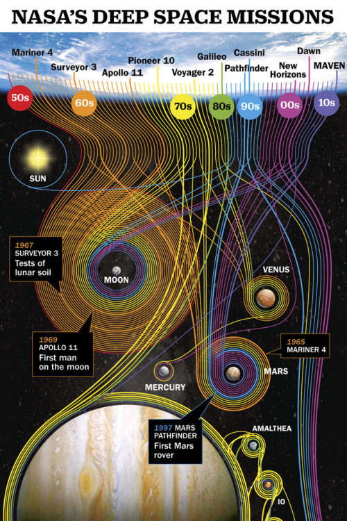
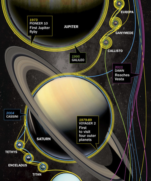
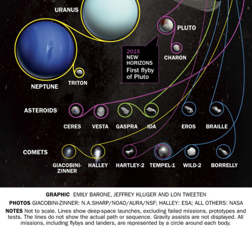
Deep Space Missions

Better Sleep tips.

Working too hard, feeling overwhelmed by family responsibilities, or dealing with an ongoing challenge? 

Maybe it’s time to turn your attention back to yourself and to your own self-care. Although we often brush it aside, self-care is not optional if you want to be happy and healthy.

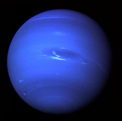
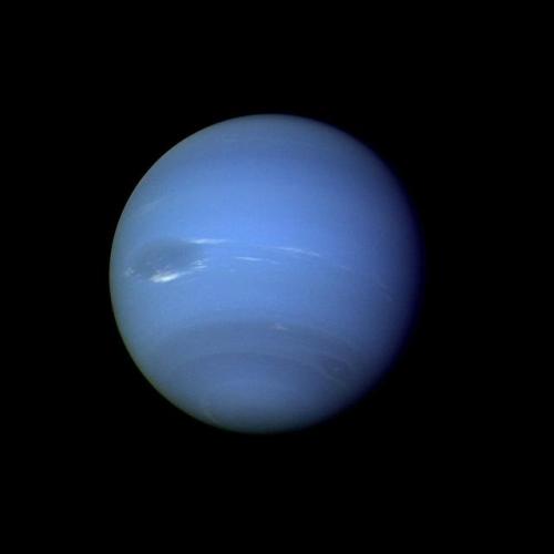
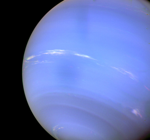
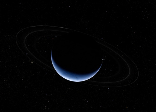
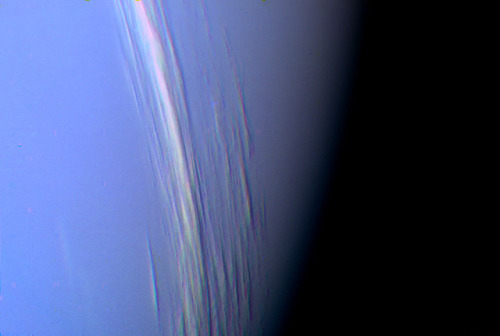
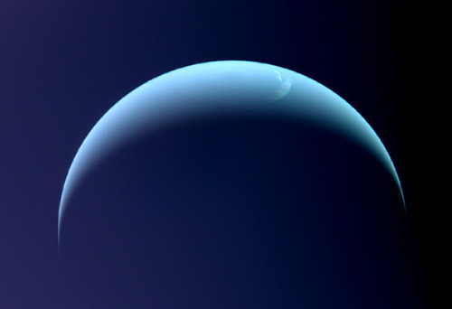
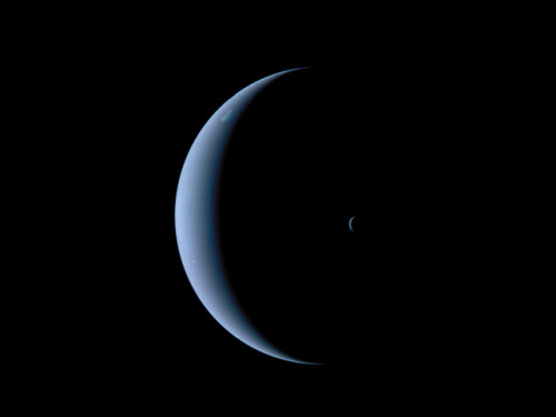
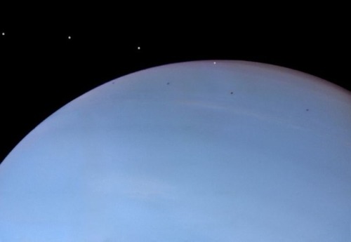
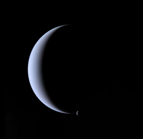
Neptune ♆

On this day in 1846 was discovered the planet Neptune.

The ice giant Neptune was the first planet located through mathematical predictions rather than through regular observations of the sky. (Galileo had recorded it as a fixed star during observations with his small telescope in 1612 and 1613.) When Uranus didn’t travel exactly as astronomers expected it to, a French mathematician, Urbain Joseph Le Verrier, proposed the position and mass of another as yet unknown planet that could cause the observed changes to Uranus’ orbit. After being ignored by French astronomers, Le Verrier sent his predictions to Johann Gottfried Galle at the Berlin Observatory, who found Neptune on his first night of searching in 1846. Seventeen days later, its largest moon, Triton, was also discovered.

Neptune is invisible to the naked eye because of its extreme distance from Earth. Interestingly, the highly eccentric orbit of the dwarf planet Pluto brings Pluto inside Neptune’s orbit for a 20-year period out of every 248 Earth years. Pluto can never crash into Neptune, though, because for every three laps Neptune takes around the Sun, Pluto makes two. This repeating pattern prevents close approaches of the two bodies.

Nearly 4.5 billion kilometers (2.8 billion miles) from the Sun, Neptune orbits the Sun once every 165 years. 

Uranus’ blue-green color is also the result of atmospheric methane, but Neptune is a more vivid, brighter blue, so there must be an unknown component that causes the more intense color. 

Despite its great distance and low energy input from the Sun, Neptune’s winds can be three times stronger than Jupiter’s and nine times stronger than Earth’s.

Winds on Neptune travel faster than the speed of sound.

In 1989, Voyager 2 tracked a large, oval-shaped, dark storm in Neptune’s southern hemisphere. This “Great Dark Spot” was large enough to contain the entire Earth.

Neptune has five known rings. Voyager 2’s observations confirmed that these unusual rings are not uniform but have four thick regions (clumps of dust) called arcs. The rings are thought to be relatively young and short-lived.

Neptune has 14 known moons, six of which were discovered by Voyager 2.

Triton, Neptune’s largest moon, orbits the planet in the opposite direction compared with the rest of the moons, suggesting that it may have been captured by Neptune in the distant past. 

To know more about the planet Neptune click here and here.

Images credit: NASA/JPL- Caltech (some images processed by Kevin M. Gill)

If the Moon were replaced with some of our planets (at night)

Image credit: yeti dynamics

Cosmic rays

Cosmic rays provide one of our few direct samples of matter from outside the solar system. They are high energy particles that move through space at nearly the speed of light. Most cosmic rays are atomic nuclei stripped of their atoms with protons (hydrogen nuclei) being the most abundant type but nuclei of elements as heavy as lead have been measured. Within cosmic-rays however we also find other sub-atomic particles like neutrons electrons and neutrinos.

Since cosmic rays are charged – positively charged protons or nuclei, or negatively charged electrons – their paths through space can be deflected by magnetic fields (except for the highest energy cosmic rays). On their journey to Earth, the magnetic fields of the galaxy, the solar system, and the Earth scramble their flight paths so much that we can no longer know exactly where they came from. That means we have to determine where cosmic rays come from by indirect means.

Because cosmic rays carry electric charge, their direction changes as they travel through magnetic fields. By the time the particles reach us, their paths are completely scrambled, as shown by the blue path. We can’t trace them back to their sources. Light travels to us straight from their sources, as shown by the purple path.

One way we learn about cosmic rays is by studying their composition. What are they made of? What fraction are electrons? protons (often referred to as hydrogen nuclei)? helium nuclei? other nuclei from elements on the periodic table? Measuring the quantity of each different element is relatively easy, since the different charges of each nucleus give very different signatures. Harder to measure, but a better fingerprint, is the isotopic composition (nuclei of the same element but with different numbers of neutrons). To tell the isotopes apart involves, in effect, weighing each atomic nucleus that enters the cosmic ray detector.

All of the natural elements in the periodic table are present in cosmic rays. This includes elements lighter than iron, which are produced in stars, and heavier elements that are produced in violent conditions, such as a supernova at the end of a massive star’s life.

Detailed differences in their abundances can tell us about cosmic ray sources and their trip through the galaxy. About 90% of the cosmic ray nuclei are hydrogen (protons), about 9% are helium (alpha particles), and all of the rest of the elements make up only 1%. Even in this one percent there are very rare elements and isotopes. Elements heavier than iron are significantly more rare in the cosmic-ray flux but measuring them yields critical information to understand the source material and acceleration of cosmic rays.

Even if we can’t trace cosmic rays directly to a source, they can still tell us about cosmic objects. Most galactic cosmic rays are probably accelerated in the blast waves of supernova remnants. The remnants of the explosions – expanding clouds of gas and magnetic field – can last for thousands of years, and this is where cosmic rays are accelerated. Bouncing back and forth in the magnetic field of the remnant randomly lets some of the particles gain energy, and become cosmic rays. Eventually they build up enough speed that the remnant can no longer contain them, and they escape into the galaxy.

Cosmic rays accelerated in supernova remnants can only reach a certain maximum energy, which depends on the size of the acceleration region and the magnetic field strength. However, cosmic rays have been observed at much higher energies than supernova remnants can generate, and where these ultra-high-energies come from is an open big question in astronomy. Perhaps they come from outside the galaxy, from active galactic nuclei, quasars or gamma ray bursts.

Or perhaps they’re the signature of some exotic new physics: superstrings, exotic dark matter, strongly-interacting neutrinos, or topological defects in the very structure of the universe. Questions like these tie cosmic-ray astrophysics to basic particle physics and the fundamental nature of the universe. (source)

(Source)

(Source)

(Source)

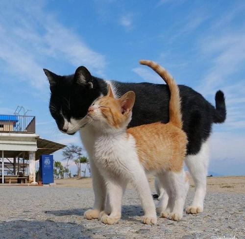
Couple goals

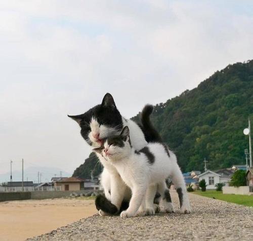
(Source)

Take me back to California 🌴❤️

I love flowers 💐❤️

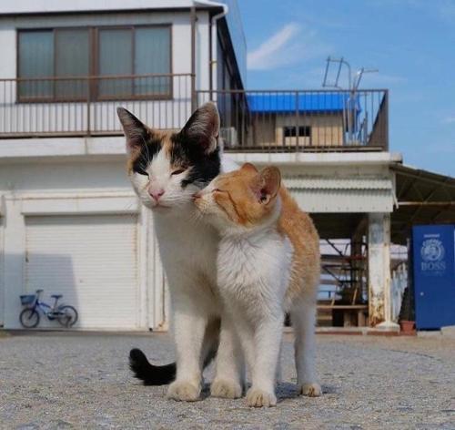
All cats are beautiful 🐱❤️

I love the sky colors ☀️ 🌤❤️

I love baby huskies ❤️

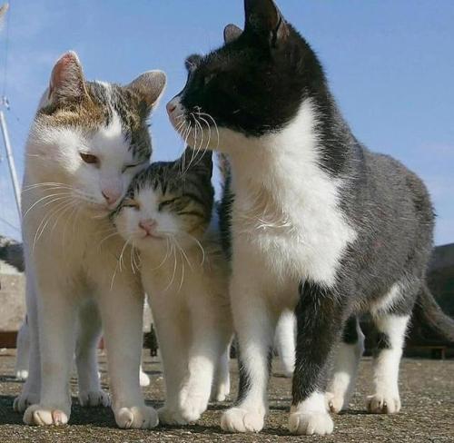
All cats are beautiful 🐱❤️

How Do You Like Your Turkey? Home-Cooked or Rocket-Launched?

It’s Thanksgiving, which means that you’re probably thinking about food right now. And here at NASA, we have to think about food very seriously when we explore space!

Astronauts Need to Eat, Too!

Like for you on Earth, nutrition plays a key role in maintaining the health and optimal performance of the astronauts. The Space Food Systems team is required to meet the nutritional needs of each crew member while adhering to the requirements of limited storage space, limited preparation options, and the difficulties of eating without gravity. 

Good food is necessary being comfortable on a mission a long way from home — especially for crewmembers who are on board for many months at a time. It’s important that the astronauts like the food they’re eating everyday, even given the preparation constraints!

Astronaut Food Has Not Always Been Appetizing

The early space programs were groundbreaking in a lot of ways — but not when it came to food. Like today, crumbs had to be prevented from scattering in microgravity and interfering with the instruments. Mercury astronauts had to endure bite-sized cubes, freeze-dried powders, and semi-liquids stuffed into aluminum tubes. The freeze-dried food were hard to rehydrate, squeezing the tubes was understandable unappetizing, and the food was generally considered to be, like spaceflight, a test of endurance.

However, over the years, packaging improved, which in turn enhanced food quality and choices. The Apollo astronauts were the first to have hot water, which made rehydrating foods easier and improved the food’s taste. And even the Space Shuttle astronauts had opportunities to design their own menus and choose foods commercially available on grocery store shelves. 

 The Wonders of Modern Space Food

Nowadays, astronauts on the International Space Station have the opportunity to sample a variety of foods and beverages prepared by the Space Food Systems team and decide which ones they prefer. They can add water to rehydratable products or eat products that are ready to eat off the shelf.

All the cooking and preparation has been done for them ahead of time because 1) they don’t have room for a kitchen to cook on the space station 2) they don’t have time to cook! The crewmembers are extremely occupied with station maintenance as well as scientific research on board, so meal times have to be streamlined as much as possible. 

Instead of going grocery shopping, bulk overwrap bags (BOBs!) are packed into cargo transfer bags for delivery to the space station. Meal based packaging allows the astronauts to have entrees, side dishes, snacks, and desserts to choose from. 

Taste in Space

The perception of taste changes in space. In microgravity, astronauts experience a fluid shift in their bodies, so the sensation is similar to eating with a headcold. The taste is muted so crewmembers prefer spicy foods or food with condiments to enhance the flavor. 

We Can’t Buy Groceries, But We Can Grow Food!

Growing plants aboard the space station provides a unique opportunity to study how plants adapt to microgravity. Plants may serve as a food source for long term missions, so it’s critical to understand how spaceflight affects plant growth. Plus, having fresh food available in space can have a positive impact on astronauts’ moods!

Since 2002, the Lada greenhouse has been used to perform almost continuous plant growth experiments on the station. We have grown a vast variety of plants, including thale cress, swiss chard, cabbage, lettuce, and mizuna. 

And in 2015, Expedition 44 members became the first American astronauts to eat plants grown in space when they munched on their harvest of Red Romaine. 

Earthlings Can Eat Space Food, Too

To give you a clear idea of how diverse the selection is for astronauts on board the space station, two earthlings gave the astronaut menu a try for a full week. Besides mentioning once that hot sauce was needed, they fared pretty well! (The shrimp cocktail was a favorite.)

Space Technology for Food on Earth

Not only has our space food improved, but so has our ability measure food production on Earth. Weather that is too dry, too wet, too hot, or too cool can strongly affect a farmer’s ability to grow crops. We collaborated with the United States Agency for International Development to create a system for crop yield prediction based on satellite data: the GEOGLAM Crop Monitor for Early Warning.

This map measures the health, or “greenness” of vegetation based on how much red or near-infrared light the leaves reflect. Healthy vegetation reflects more infrared light and less visible light than stressed vegetation. As you can see from the map, a severe drought spread across southern Mexico to Panama in June to August of this year. 

The Crop Monitor compiles different types of crop condition indicators — such as temperature, precipitation, and soil moisture — and shares them with 14 national and international partners to inform relief efforts.

Thanksgiving in Space 

Space food has certainly come a long way from semi-liquids squeezed into aluminum tubes! This year, Expedition 57 crewmembers Commander Alexander Gerst and Flight Engineer Serena M. Auñón-Chancellor are looking forward to enjoying a Thanksgiving meal that probably sounds pretty familiar to you: turkey, stuffing, candied yams, and even spicy pound cakes!

Hungry for More?

If you can’t get enough of space food, tune into this episode of “Houston, We Have a Podcast” and explore the delicious science of astronaut mealtime with Takiyah Sirmons. 

And whether you’re eating like a king or an astronaut, we wish everybody a happy and safe Thanksgiving!

11/08/18

Jovian Close Encounter

A multitude of magnificent, swirling clouds in Jupiter’s dynamic North North Temperate Belt is captured in this image from NASA’s Juno spacecraft. Appearing in the scene are several bright-white “pop-up” clouds as well as an anticyclonic storm, known as a white oval. This color-enhanced image was taken at 1:58 p.m. PDT on Oct. 29, 2018 (4:58 p.m. EDT) as the spacecraft performed its 16th close flyby of Jupiter. At the time, Juno was about 4,400 miles (7,000 kilometers) from the planet’s cloud tops, at a latitude of approximately 40 degrees north. Citizen scientists Gerald Eichstädt and Seán Doran created this image using data from the spacecraft’s JunoCam imager. JunoCam’s raw images are available for the public to peruse and to process into image products at: http://missionjuno.swri.edu/junocam.

During its continued mission, NASA’s Juno spacecraft will maintain its 53-day polar orbit around Jupiter. At its closest, Juno passes within 3,000 miles (5,000 kilometers) of Jupiter’s cloud tops once during each 53-day orbit. At the high end of each orbit, Juno is about 5 million miles (8-million kilometers) from the planet – which is just beyond the orbit of the Jovian moon Themisto. Credits: NASA/JPL-Caltec